Canonical Correlation Analysis (CCA) in R
What is CCA? Link to heading
When our statistician recommended we use a CCA on our data, I have to admit I had never heard of it before. I was surprised to find out that it is a very powerful alternative to running several multivariate regressions or dimension reduction techniques like Principal Component Analysis (PCA) or Independent Component Analysis (ICA), which can sometimes be challenging to interpret.
Canonical Correlation Analysis (CCA) is similar to PCA, but with some important differences. Whereas PCA finds the direction accounting for most of the observed variance in a single high-dimensional variable set – CCA finds the direction accounting for most of the covariance between two high-dimensional variable sets. Thus, CCA might be the appropriate test for you if you are interested in exploring multivariate associations between two variable sets, dimension reduction and/or feature selection. Both PCA and CCA was developed by Harold Hotelling in the 1930’s. In other words, CCA is not a new statistical method, although I see an increase in its use in my own field of research.
How does it work? Link to heading
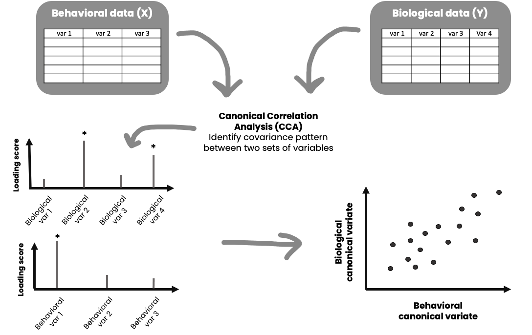
The illustration above gives you a general idea of how it works. CCA generates linear combinations of variables from two sets of variables (variable set “X” and variable set “Y”). The variables in each set usually have something in common, for instance it could be that variables in set X are different behavioral measures, and variables in set Y are different biological measures. These new variables, the linear combinations, are called canonical variates. These canonical variates form different modes (similar to components in PCA) of covariation (canonical variate pairs), and the correlation between them is called a canonical correlation. The maximum number of possible modes of covariation equals the number of variables in the smallest variable set. For instance, if variable set X has 10 variables, and variable set Y has 16 variables, it is possible to have 10 significant modes of covariation – each capturing different aspects of your data.
If you are like me you also think this is complicated stuff. Lets break it down with an example.
- You submit variable set X (10 variables) and variable set Y (16 variables) to a CCA
- The CCA generates 10 canonical correlations (correlation between different linear combinations of your variable sets) as you have 10 possible modes of covariation
- You run tests to find out how many and which modes are significant (lets say the first two are significant)
- Then you want to assess which of the variables in each set is driving the correlation for each significant mode (check the loading of each variable, which is its correlation to the corresponding canonical variate)
- Each individual gets assigned a loading score for the X and Y canonical variates for each mode
- You can then for example do further tests investigating whether there are differences between different defining features of these individuals (i.e. diagnosis vs. no diagnosis) on their loading scores
- You can also use the CCA for feature selection and dimension reduction, i.e. lets say a mode captures variable 2,3, and 6 in variable set X and variable 7 and 8 in variable set Y that explains most of the variance in your data, and you might want to only focus on these in subsequent analyses
What are the assumptions of CCA? Link to heading
CCA assumes multivariate normality, and require a decent subject-to-variable ratio (SVR) in order to produce stable and reliable results. I recommend you check out https://www.uaq.mx/statsoft/stcanan.html#assumptions for a general description, and Yang et al., (2023) for details. Ideally, you should have more observations/subjects than variables.
CCA tutorial Link to heading
Packages and data
We will use the function cancor in the candisc package to run CCA. This tutorial also uses the tidyverse. First, lets load the packages we need:
#### ---- Load packages ---- ####
library(candisc)
library(tidyverse)
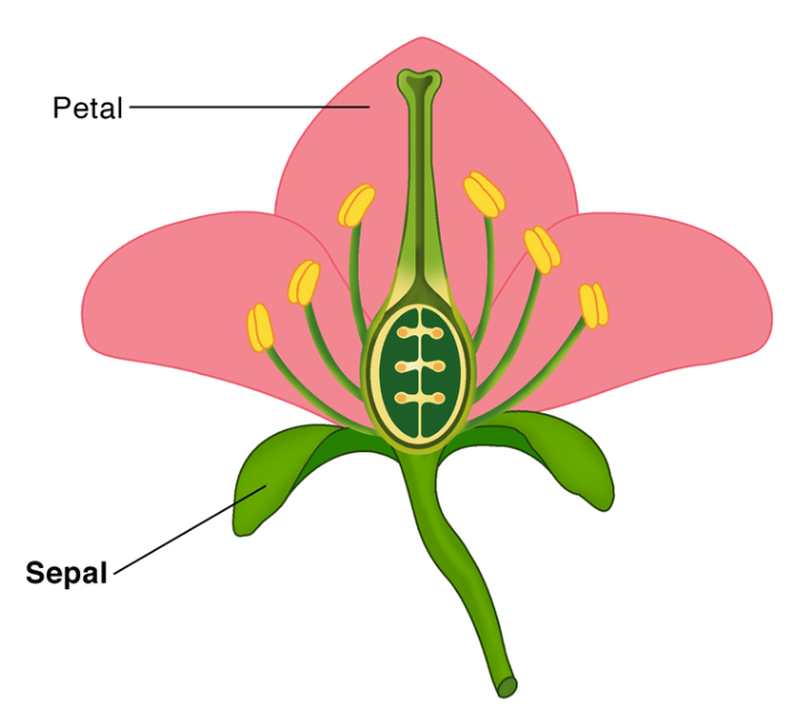
For this tutorial we will be using the iris dataset. The dataset consists of measurements of different features of three Iris species – setosa, virginica, and versicolor. A fun fact for you is that are up to 280 species of Iris on the planet. The measurements include the length and width (in cm) of the sepals and petals of the flower. In case you are confused, look at the image below for what petals and sepals are, borrowed from ScienceFacts.net.
This is how you load the data:
#### ---- Load data ---- ####
data(iris)
Lets have a look at the first rows:
head(iris)
  Sepal.Length Sepal.Width Petal.Length Petal.Width Species
1          5.1         3.5          1.4         0.2  setosa
2          4.9         3.0          1.4         0.2  setosa
3          4.7         3.2          1.3         0.2  setosa
4          4.6         3.1          1.5         0.2  setosa
5          5.0         3.6          1.4         0.2  setosa
6          5.4         3.9          1.7         0.4  setosa
And also lets have a look at some descriptives:
summary(iris)
  Sepal.Length    Sepal.Width     Petal.Length    Petal.Width
 Min.   :4.300   Min.   :2.000   Min.   :1.000   Min.   :0.100
 1st Qu.:5.100   1st Qu.:2.800   1st Qu.:1.600   1st Qu.:0.300
 Median :5.800   Median :3.000   Median :4.350   Median :1.300
 Mean   :5.843   Mean   :3.057   Mean   :3.758   Mean   :1.199
 3rd Qu.:6.400   3rd Qu.:3.300   3rd Qu.:5.100   3rd Qu.:1.800
 Max.   :7.900   Max.   :4.400   Max.   :6.900   Max.   :2.500
       Species
 setosa    :50
 versicolor:50
 virginica :50
Data preparation
If you have lots of variables in each variable set, it can be a good idea to apply some dimension reduction before you begin (for instance a PCA, and use the first component explaining most of the variance). However, keep in mind that this can further challenge interpretation and reproducibility (Dinga et al., 2019). A good practice for CCA is to standardize the data (Z-scores), so that they have a mean of 0 and a standard deviation of 1. Lets do that.
#### ---- Standardize numeric variables using mutate and across ---- ####
iris_scaled <- iris %>%
  mutate(across(where(is.numeric), ~as.vector(scale(.)))) %>%
  setNames(names(iris))

summary(iris_scaled)
  Sepal.Length       Sepal.Width       Petal.Length      Petal.Width
 Min.   :-1.86378   Min.   :-2.4258   Min.   :-1.5623   Min.   :-1.4422
 1st Qu.:-0.89767   1st Qu.:-0.5904   1st Qu.:-1.2225   1st Qu.:-1.1799
 Median :-0.05233   Median :-0.1315   Median : 0.3354   Median : 0.1321
 Mean   : 0.00000   Mean   : 0.0000   Mean   : 0.0000   Mean   : 0.0000
 3rd Qu.: 0.67225   3rd Qu.: 0.5567   3rd Qu.: 0.7602   3rd Qu.: 0.7880
 Max.   : 2.48370   Max.   : 3.0805   Max.   : 1.7799   Max.   : 1.7064
       Species
 setosa    :50
 versicolor:50
 virginica :50
Next, we want to define our X and Y variable sets. Here I will use sepal length and width as the X variables and petal length and width as the Y variables. We will save the species variable for later so we can see whether the CCA captures differences in these species.
#### ---- Define X and Y variable sets ---- ####
X <- iris_scaled %>%
  select(Sepal.Length, Sepal.Width)


Y <- iris_scaled %>%
  select(Petal.Length, Petal.Width)

head(X)
  Sepal.Length Sepal.Width
1   -0.8976739  1.01560199
2   -1.1392005 -0.13153881
3   -1.3807271  0.32731751
4   -1.5014904  0.09788935
5   -1.0184372  1.24503015
6   -0.5353840  1.93331463
head(Y)
  Petal.Length Petal.Width
1    -1.335752   -1.311052
2    -1.335752   -1.311052
3    -1.392399   -1.311052
4    -1.279104   -1.311052
5    -1.335752   -1.311052
6    -1.165809   -1.048667
Running the CCA
Now we can run the CCA, like this:
#### ---- Run CCA ---- ####
CCA_res <- cancor(X, Y)
Lets have a look at the output of CCA_res:
CCA_res
Canonical correlation analysis of:
     2   X  variables:  Sepal.Length, Sepal.Width
  with   2   Y  variables:  Petal.Length, Petal.Width

    CanR  CanRSQ  Eigen percent   cum                          scree
1 0.9410 0.88542 7.7277 99.7985  99.8 ******************************
2 0.1239 0.01536 0.0156  0.2015 100.0

Test of H0: The canonical correlations in the
current row and all that follow are zero

     CanR LR test stat approx F numDF denDF Pr(> F)
1 0.94097      0.11282  144.338     4   292  <2e-16 ***
2 0.12394      0.98464    2.293     1   147  0.1321
---
Signif. codes:  0 '***' 0.001 '**' 0.01 '*' 0.05 '.' 0.1 ' ' 1
The canonical correlation between the first canonical variates of X and Y is very high (r=0.94), however, the second is low (r=0.12). This is shown under CanR. The next output is a test of the null hypothesis that the first set of variables is independent of the second set of variables. We can see here that the first “mode” is significant at p<0.001. Great! We only evaluate the significant mode. Now, lets have a look at interpreting our significant mode – what is it capturing?
Obtain raw canonical coefficients
You will find the raw canonical coefficients here:
CCA_res$coef$X
                  Xcan1     Xcan2
Sepal.Length -0.8851871 0.4800626
Sepal.Width   0.3726619 0.9354889
CCA_res$coef$Y
                  Ycan1     Ycan2
Petal.Length -1.4989586 -3.387093
Petal.Width   0.5288422  3.666006
Here we only evaluate the column Xcan1 since this was the only significant mode. If you have several significant modes of covariation, each one could capture different aspects of your data. The raw canonical coefficients are interpreted similarly to regression coefficients. For instance, one unit increase in the variable Sepal Length results in a 0.929 decrease in the first mode/dimension (when all other variables are held constant). However, it is easier to interpret the covariance mode if we look at the correlations between each variable and the corresponding canonical variate, sometimes referred to as the loading of each variable.
Obtain loadings of the variables
We want to see which variables in each variable set is contributing to the canonical correlation in our significant mode/component. The correlation between the original variables and their canonical variate can be obtained here:
CCA_res$structure$X.xscores
                  Xcan1     Xcan2
Sepal.Length -0.9290009 0.3700774
Sepal.Width   0.4767332 0.8790480
CCA_res$structure$Y.yscores
                  Ycan1     Ycan2
Petal.Length -0.9897548 0.1427778
Petal.Width  -0.9144533 0.4046915
For the measurements of sepals, our first mode is most strongly influenced by sepal length (-0.92). For measurements of petals, the first mode is influenced strongly by both length (-0.98) and width (-0.91) of the petals.
Extract loading scores for each observation
Let us extract the loading scores for all observations of flowers, and then do some visualizing.
#### ---- Extract loading score for all observations --- ###
CCA_X <- as.matrix(X) %*% CCA_res$coef$X[, 1]
CCA_Y <- as.matrix(Y) %*% CCA_res$coef$Y[, 1]
We can check if this matrix multiplication worked by looking looking at its correlation. It should be the same as the canonical correlation for this first mode.
cor(CCA_X, CCA_Y)
         [,1]
[1,] 0.940969
Tada! It is the same. Very good. Each flower that was measured now have a loading score for the X (sepal measurements) and Y (petal measurements) canonical variates in the first mode.
Has the CCA captured differences across Iris species?
We are now getting to the juicy part. Has the CCA captured differences across Iris species? Each Iris species has a loading score. Lets get these loadings and merge with the original data and look at some descriptives.
# Create dataframe with results
CCA_datares <- as.data.frame(cbind(CCA_X, CCA_Y)) %>%
  rename(mode1_X = V1, mode1_Y = V2)

# Combine with original iris dataframe
iris_CCA <- cbind(iris, CCA_datares)

# Lets have a look:
head(iris_CCA)
  Sepal.Length Sepal.Width Petal.Length Petal.Width Species   mode1_X  mode1_Y
1          5.1         3.5          1.4         0.2  setosa 1.1730856 1.308897
2          4.9         3.0          1.4         0.2  setosa 0.9593861 1.308897
3          4.7         3.2          1.3         0.2  setosa 1.3441807 1.393809
4          4.6         3.1          1.5         0.2  setosa 1.3655796 1.223984
5          5.0         3.6          1.4         0.2  setosa 1.3654828 1.308897
6          5.4         3.9          1.7         0.4  setosa 1.1943878 1.192920
# Get some descriptives by species
iris_CCA %>% group_by(Species) %>%
  summarise(mean_X = mean(mode1_X),
            mean_Y = mean(mode1_Y),
            sd_X = sd(mode1_X),
            sd_Y = sd(mode1_Y))
# A tibble: 3 × 5
  Species    mean_X mean_Y  sd_X  sd_Y
  <fct>       <dbl>  <dbl> <dbl> <dbl>
1 setosa      1.21   1.29  0.256 0.141
2 versicolor -0.345 -0.338 0.470 0.303
3 virginica  -0.867 -0.950 0.606 0.445
The setosa species seem to have a higher more positive loading score on both X (capturing mostly sepal length) and Y (both petal length and width), then versicolor has a more negative loading score, and virginica even more negative loading score. We know from the Iris dataset that setosa tends to have smaller sepal length, petal width and petal length, so this makes sense. It seems to me that the CCA has captured some difference between the species. Lets do some plotting, shall we?
Visualize results
# Basic scatterplot of the loading scores on the X and Y canonical variates.
iris_CCA %>%
  ggplot(aes(x = CCA_X, y = CCA_Y))+
  geom_point()
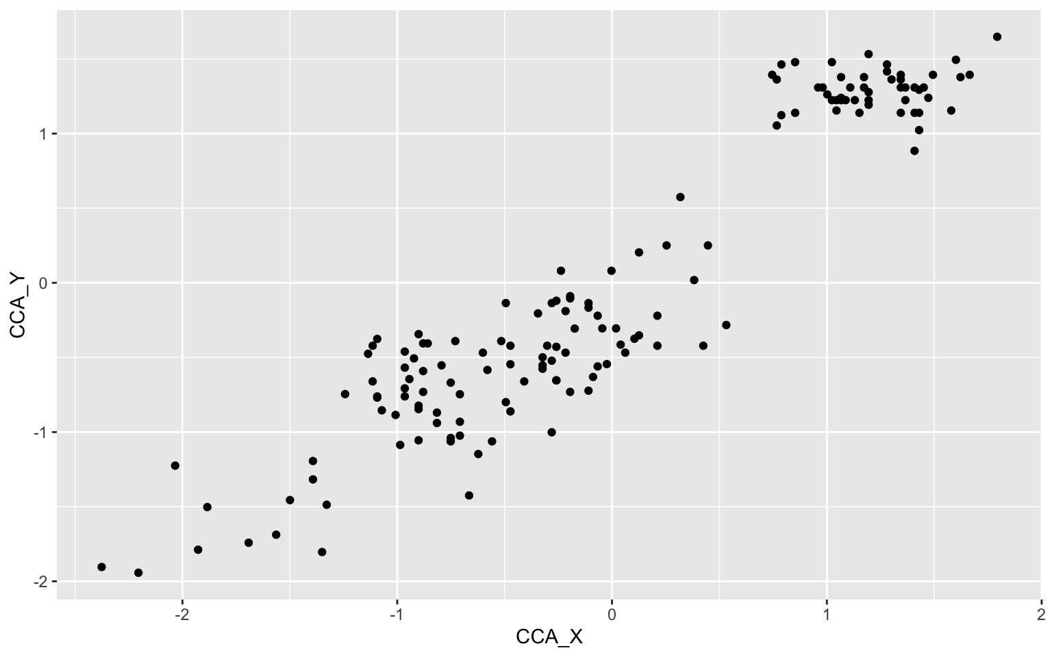
Okay, looks like we have 3 different clusters of data here maybe? Let us pimp this plot up by adding some nicer colors, a regression line, names on the axes and color the scatters by species.
# Set custom color scheme
custom_palette <- c("setosa" = "#98c1d9", "versicolor" = "#293241","virginica" = "#ee6c4d")

# Pimped plot
iris_CCA %>%
  ggplot(aes(x = CCA_X, y = CCA_Y, color = Species)) +
  geom_point(shape = 16, size = 3, alpha = 0.8) +
  geom_smooth(method = lm, color="grey", fill="grey", se = TRUE) +
  annotate("text", x = -1.7, y = -0.3, label = "r = .94", color = "#404040", size = 4, fontface = "bold") +
  labs(y = "Petal canonical variate",
       x = "Sepal canonical variate",
       color = "Species") +
  scale_color_manual(values = custom_palette) +
  theme_classic(base_size = 15)
`geom_smooth()` using formula = 'y ~ x'
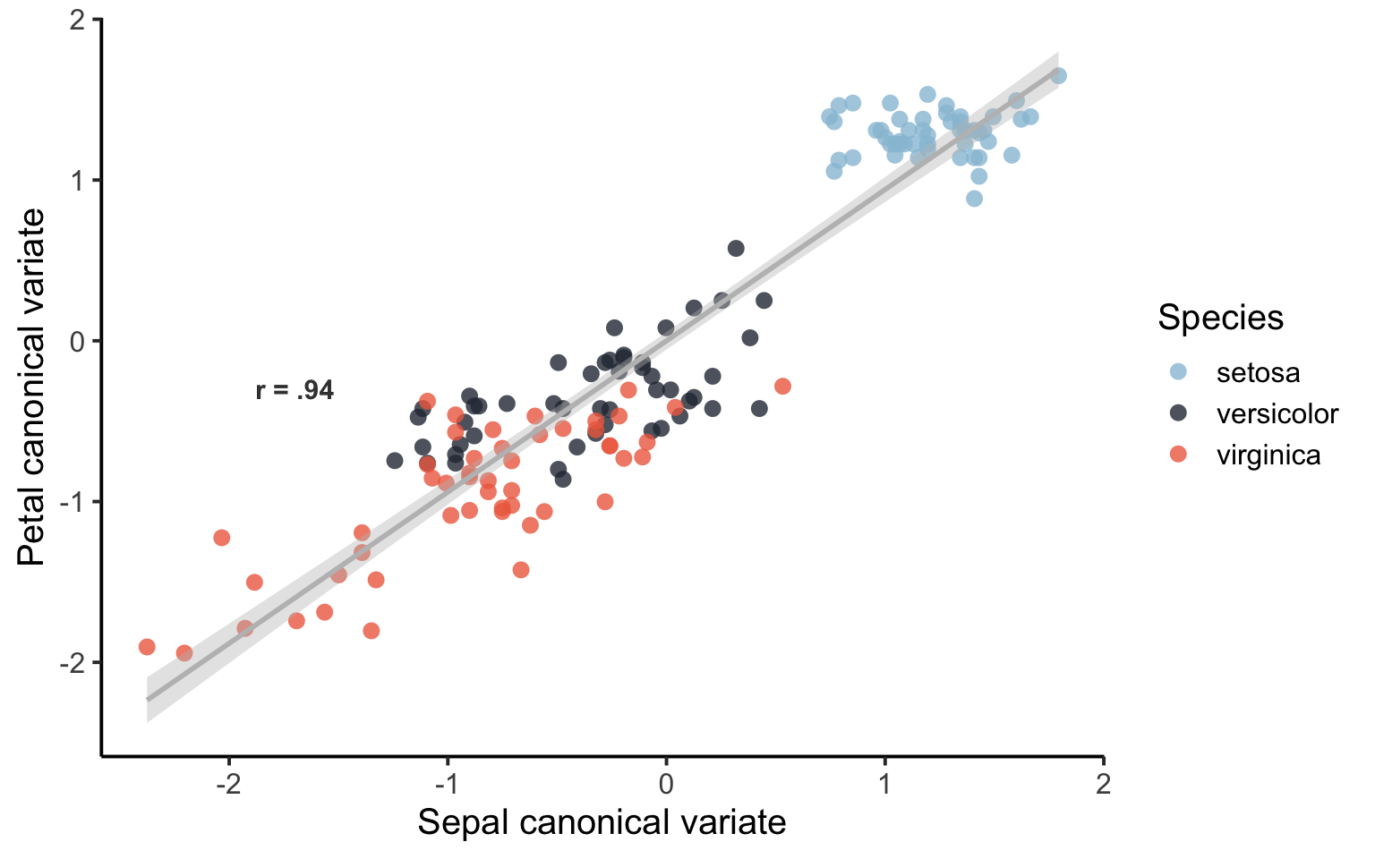
That’s a lot better. It seems like the first mode of the CCA is capturing some difference between the species of Iris. There is some overlap between versicolor and virginica. We can also have a look at the loading scores for each species of Iris in a box/violin plot:
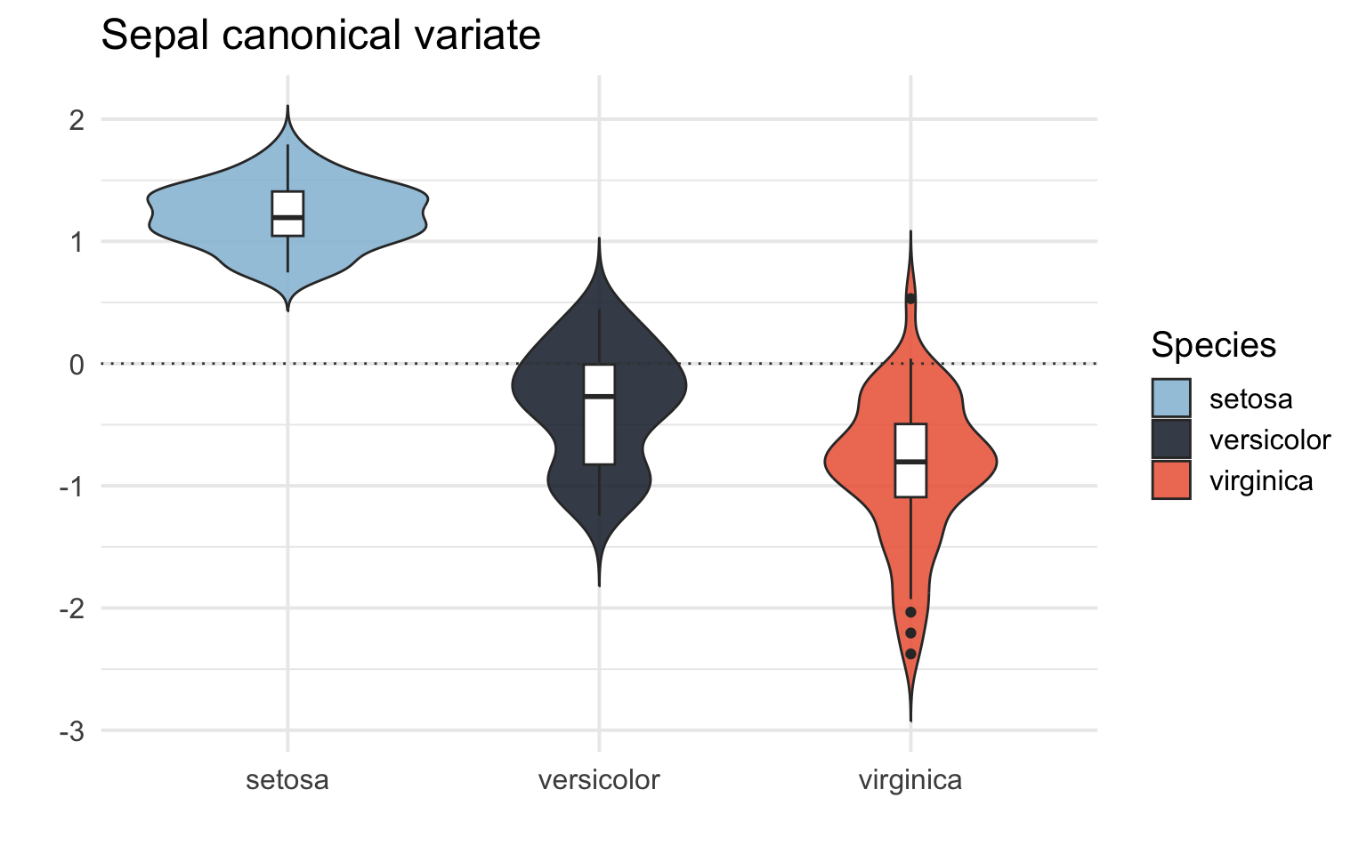
# Box/Violin plot for the sepal canonical variate (X)
iris_CCA %>%
  ggplot(aes(x = Species, y = CCA_X, fill = Species)) +
  geom_violin(trim = FALSE, alpha = 0.9) +
  geom_boxplot(width = 0.1, fill = "white") +
  geom_hline(yintercept = 0.0, color = "#404040", linetype = "dotted") +
  labs(y = "",
       title = "Sepal canonical variate",
       x = "") +
  scale_fill_manual(values = custom_palette) +
  scale_color_manual(values = custom_palette) +
  theme_minimal(base_size = 15)
# Box/Violin plot for the petal canonical variate (X)
iris_CCA %>%
  ggplot(aes(x = Species, y = CCA_Y, fill = Species)) +
  geom_violin(trim = FALSE, alpha = 0.9) +
  geom_boxplot(width = 0.1, fill = "white") +
  geom_hline(yintercept = 0.0, color = "#404040", linetype = "dotted") +
  labs(y = "",
       title = "Petal canonical variate",
       x = "") +
  scale_fill_manual(values = custom_palette) +
  scale_color_manual(values = custom_palette) +
  theme_minimal(base_size = 15)
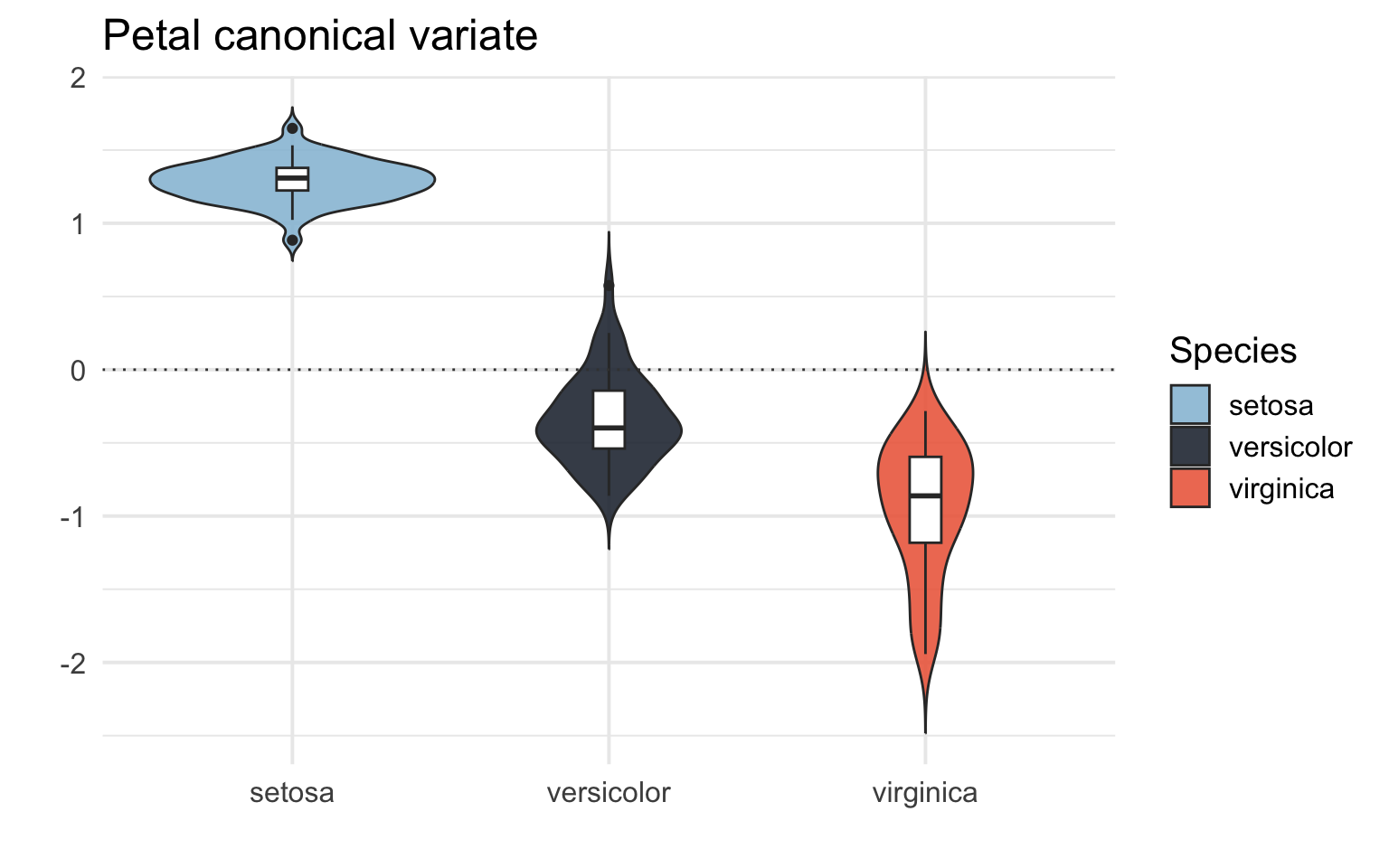
We can see that the CCA captures a difference between the different species of Iris! It tells us that different species of Iris have different patters of sepal and petal length and width.
Further reading and resources Link to heading
-
For how to report CCA in scientific publications I recommend checking out these papers from our lab and others that have used CCA, some have published the analysis code: Sæther et al., (2022), Voldsbekk et al., (2023), Fernandez-Cabello et al., (2022), and Dinga et al., (2019).
-
Here are some tutorials I found useful: cmdlinetips tutorial using tidyverse, UCLA tutorial using base R, Medium tutorial using base R.
-
I also found this SAS tutorial useful in explaining the different outputs from the CCA: SAS tutorial